5.2.31 probability distribution

The random variable X is the crew size of a randomly selected shuttle mission. Its probability distribution is shown below. Complete parts a through c.

---

data <- read.csv("https://raw.githubusercontent.com/sileaderwt/MTH1320-UMSL/main/Image%2BData/5.2.31%20%20probability%20distribution/5.2.31.csv")
data

##   x P.X.x.
## 1 2  0.034
## 2 3  0.013
## 3 4  0.072
## 4 5  0.338
## 5 6  0.210
## 6 7  0.289
## 7 8  0.044

We store data into two variables x and P

x = data$x
x

## [1] 2 3 4 5 6 7 8

P = data$P.X.x.
P

## [1] 0.034 0.013 0.072 0.338 0.210 0.289 0.044

---

(a). Find and interpret the mean of the random variable.

mu = sum(x*P)
mu

## [1] 5.72

Round to three decimal places

round(mu, 3)

## [1] 5.72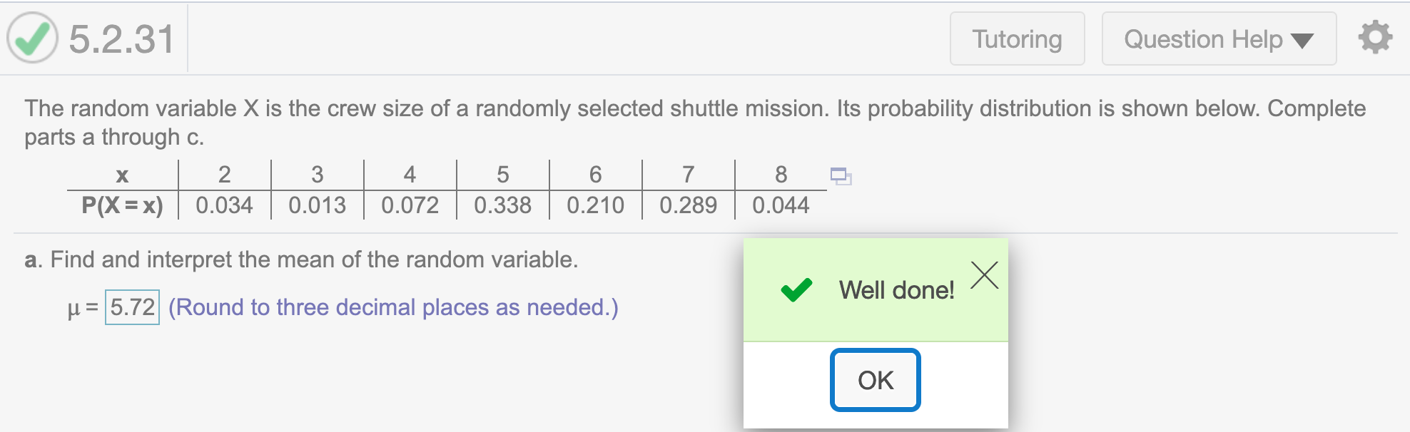

---

---

---

(b). Obtain the standard deviation of the random variable.

We can find standard deviation by using formula \(\sigma=\sqrt{\sum(x-\mu)^2P(X=x)}\)

sigma = sqrt(sum((x-mu)^2*P))
sigma

## [1] 1.293677

Round to three decimal places

round(sigma, 3)

## [1] 1.294

---

We can use alternative formula to find standarad deviation \(\sigma=\sqrt{\sum x^2P(X=x)- \mu^2}\)

sigma2 = sqrt(sum(x^2*P)-mu^2)
sigma2

## [1] 1.293677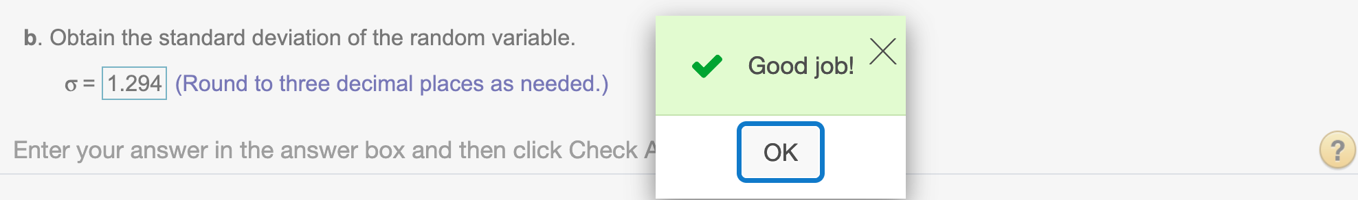

---

---

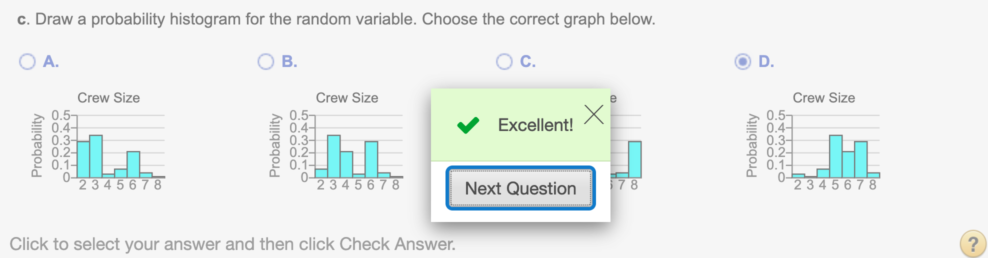
(c). Draw a probability histogram for the random variable. Choose the correct graph below.

barplot(P, names.arg = x)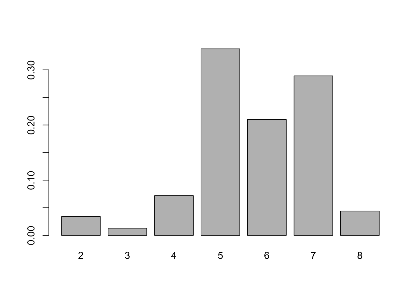

---

---

Hope that helps!