13.5.103 chi squared test with data
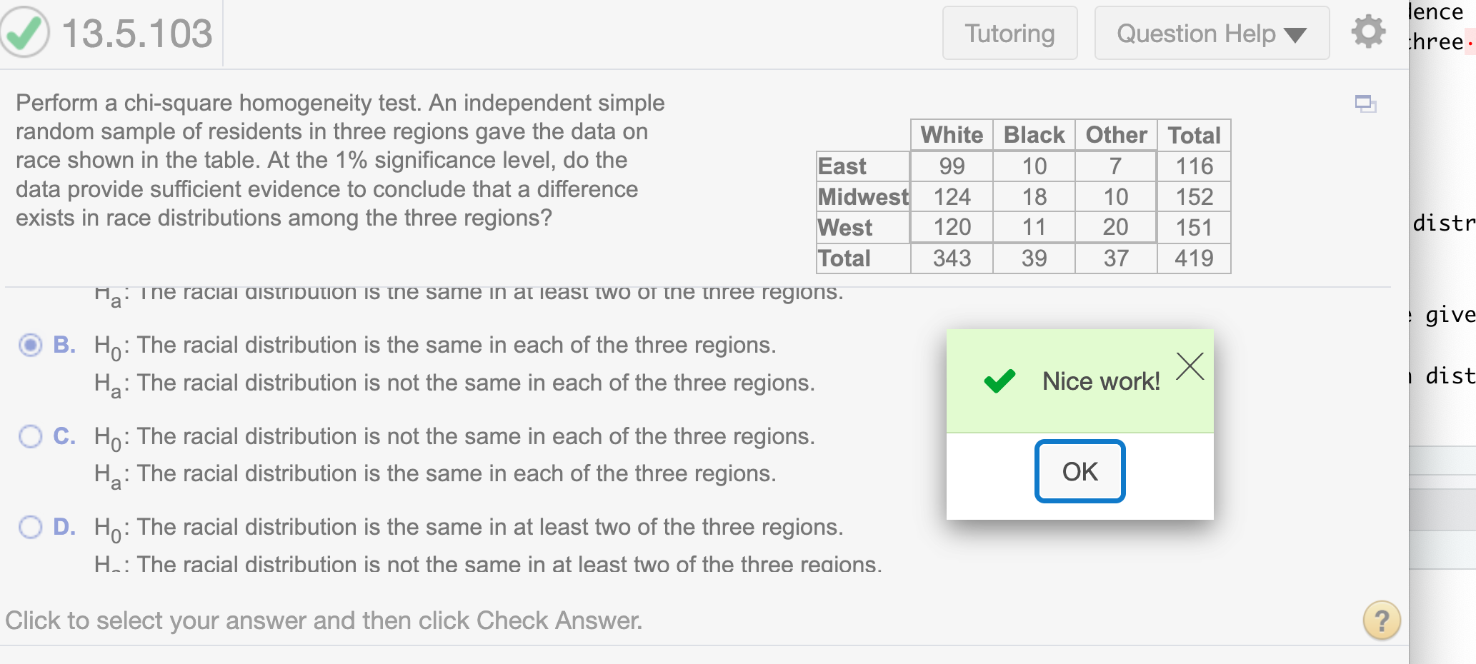
Perform a chi-square homogeneity test. An independent simple random sample of residents in three regions gave the data on race shown in the table. At the 1 % significance level, do the data provide sufficient evidence to conclude that a difference exists in race distributions among the three regions?
Name of variables
row total: rTotal
column total: cTotal
total numbers of data: total
original data: dframe1
expected frequencies data: dframe2
What are the null and alternative hypotheses?
Since the question asks “that a difference exists in race distributions among the three regions,” the correct hypothesis is
\(H_0:\) The racial distribution is the same in each of the three regions.
\(H_a:\) The racial distribution is not the same in each of the three regions.
Find the test statistic.,\(\chi^2\)
First we need to get the data from the question. (We can import it from Excel)
data <- read.csv("https://raw.githubusercontent.com/sileaderwt/MTH1320-UMSL/main/Image%2BData/13.5.103/13.5.103.csv")
data
## X. White Black Other
## 1 East 99 10 7
## 2 Midwest 124 18 10
## 3 West 120 11 20We store data into 2 different frame. The first one shows original data. The second shows expected frequency.
dframe1 = data.frame(data)
dframe2 = data.frame(data)
Conditions to run a chi-square test
All expected frequencies are 1 or greater
At most 20% of the expected frequencies are less than 5
The sample is a simple random sample
The sample is an independent sample
First approach: using chisq() in R which professor Covert introduces in the video lectures.(Recommended)
This approach is cleaner and faster
First we need to create a new data frame which does not contain a column of names so our data frame only contains data.
We can use subset to drop column of name.
dframe3 = subset(dframe1, select = -c(X.))
dframe3
## White Black Other
## 1 99 10 7
## 2 124 18 10
## 3 120 11 20To see the difference between dframe1 and dframe3, we can run
dframe1## X. White Black Other
## 1 East 99 10 7
## 2 Midwest 124 18 10
## 3 West 120 11 20We run chisq.test()
chisq.test(dframe3, correct=FALSE)##
## Pearson's Chi-squared test
##
## data: dframe3
## X-squared = 7.2825, df = 4, p-value = 0.1217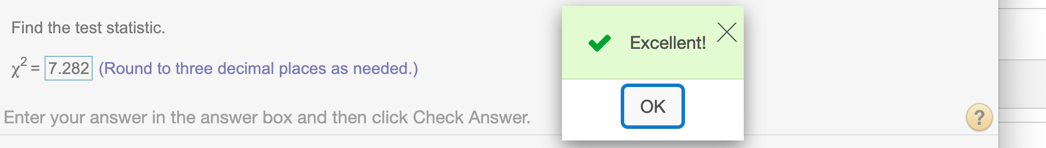
Since df = 4, to find critical value for \(\alpha = .01\)
alpha = .01
round(qchisq(1- alpha,4),3)
## [1] 13.277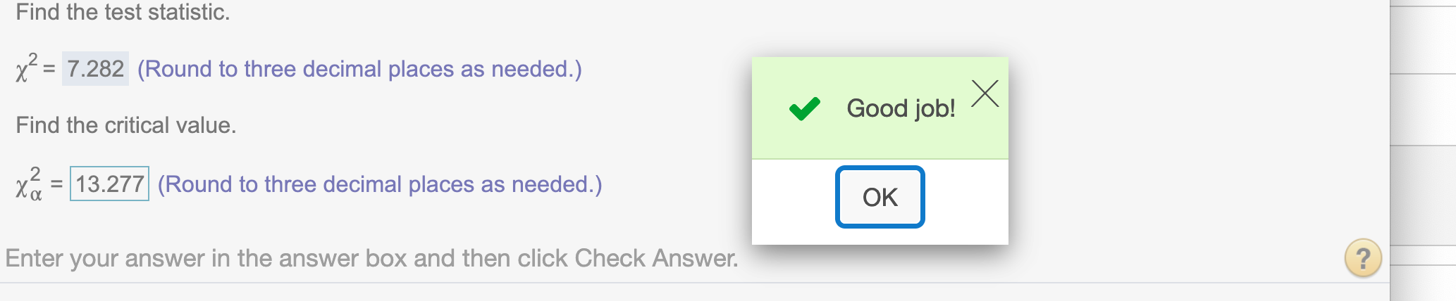
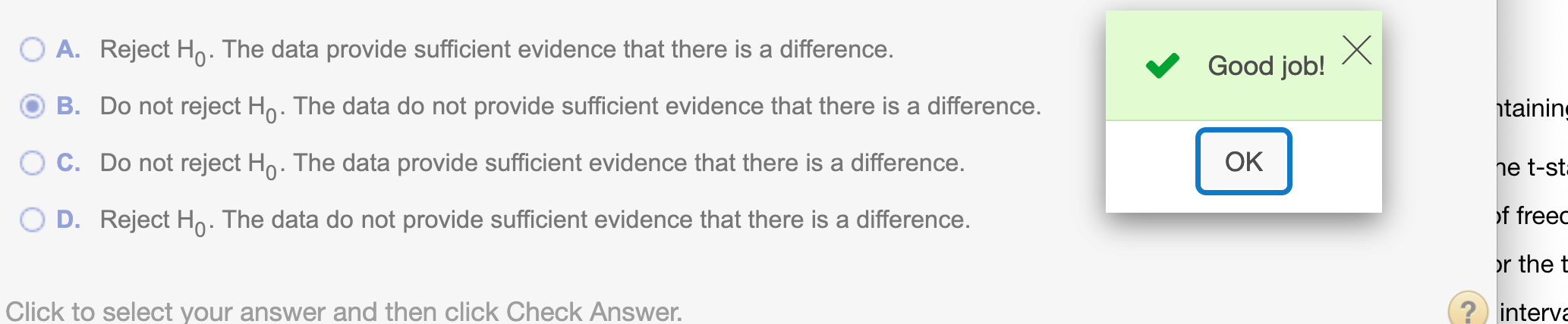
Since \(\chi^2\) is right-tailed test by nature, our test statistic does not lie in rejected region 7.282 < 13.277 , we do not have enough evidence to reject the hypothesis
If the question ask about expected frequencies, we can find it by running
chisq.test(dframe3, correct=FALSE)$expected## White Black Other
## 1 94.95943 10.79714 10.24344
## 2 124.42959 14.14797 13.42243
## 3 123.61098 14.05489 13.33413Second approach using formular
First we need to find row total and column total.
cTotal = rep(0, nrow(dframe2))
rTotal = c()
for (i in 2:ncol(dframe2)){
  cTotal = cTotal + dframe2[,i]
  rTotal = c(rTotal, sum(dframe2[,i]))
}
total = sum(cTotal)cTotal## [1] 116 152 151rTotal## [1] 343 39 37total## [1] 419We can find the test statistic \(\chi^2\) by using the formula \(\chi^2=\sum{\frac{(O-E)^2}{E}}\)
for (i in 2:ncol(dframe2)){
  dframe2[,i] <- sum(dframe2[,i])*cTotal/total
  print(dframe2[,i])
}
## [1] 94.95943 124.42959 123.61098
## [1] 10.79714 14.14797 14.05489
## [1] 10.24344 13.42243 13.33413dframe2## X. White Black Other
## 1 East 94.95943 10.79714 10.24344
## 2 Midwest 124.42959 14.14797 13.42243
## 3 West 123.61098 14.05489 13.33413Find the test statistic.,\(\chi^2\)
chi = 0
for (i in 2:ncol(dframe2)){
  chi = chi + sum((dframe1[,i]-dframe2[,i])^2/dframe2[,i])
}
chi
## [1] 7.282498Round to three decimal places
round(chi,3)## [1] 7.282Find the critical value.\(\chi_{\alpha}^2\)
We find degree of freedom by using the formula \(df=(r-1)(c-1)\)
Since dframe2 has 4 variables and the first one is x, so ncol(dframe2) returns 1 more than actual value. We find degree of freedom by running
df = (ncol(dframe2)-2) * (nrow(dframe2)-1)
df
## [1] 4Our significant level is 1%, so \(\alpha = .01\)
alpha = .01
round(qchisq(1- alpha,df),3)
## [1] 13.277Hope that helps!