13.4.75 expected frequencies
The contingency table shown to the right gives a cross-classification of a random sample of values for two variables, x and y, of a population.
First we need to get the data from the question. (We can import it from Excel)
data <- read.csv("https://raw.githubusercontent.com/sileaderwt/MTH1320-UMSL/main/Image%2BData/13.4.75/13.4.75.csv")
data
## X A B
## 1 a 50 20
## 2 b 10 40We store data into dframe
dframe = data.frame(data)
dframe
## X A B
## 1 a 50 20
## 2 b 10 40Conditions to run a chi-square test
All expected frequencies are 1 or greater
At most 20% of the expected frequencies are less than 5
The sample is a simple random sample
The sample is an independent sample
(a). Compute the expected frequencies and add them into the table given below.
First we need to create a new data frame which does not contain a column of names so our data frame only contains data.
We can use subset to drop column of name.
dframe2 = subset(dframe, select = -c(X))
dframe2
## A B
## 1 50 20
## 2 10 40To see the difference between dframe and dframe2, we can run
dframe## X A B
## 1 a 50 20
## 2 b 10 40To find expected frequencies, we can run
chisq.test(dframe2, correct=FALSE)$expected## A B
## 1 35 35
## 2 25 25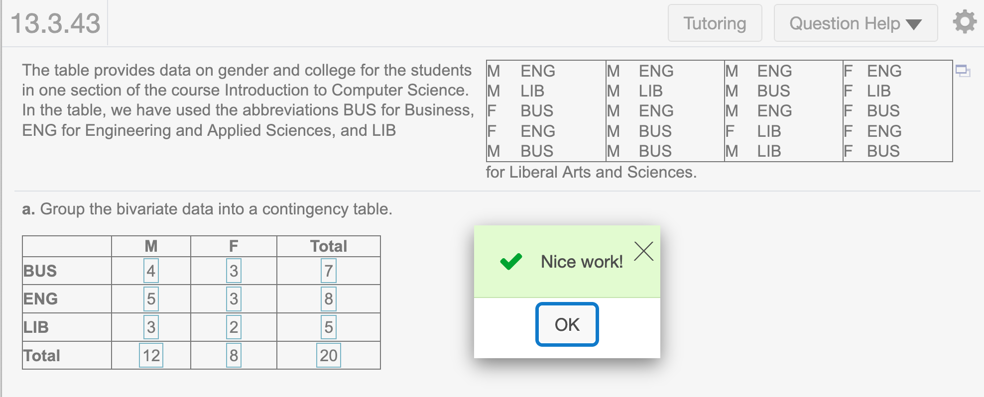
b. The test statistic is
We run chisq.test()
chisq.test(dframe2, correct=FALSE)##
## Pearson's Chi-squared test
##
## data: dframe2
## X-squared = 30.857, df = 1, p-value = 2.777e-08round(chisq.test(dframe2, correct=FALSE)$statistic,2)## X-squared
## 30.86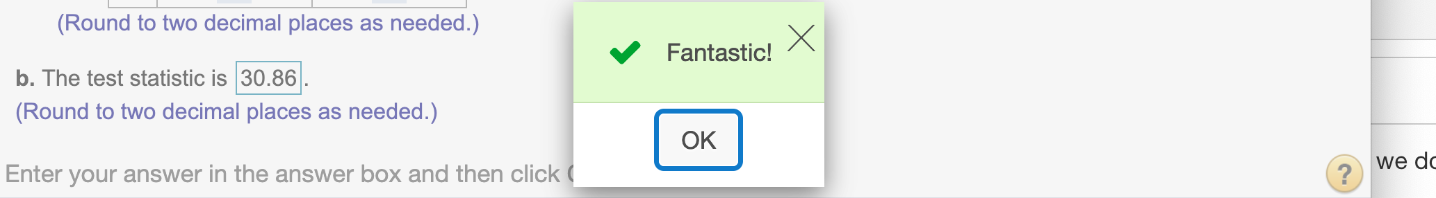
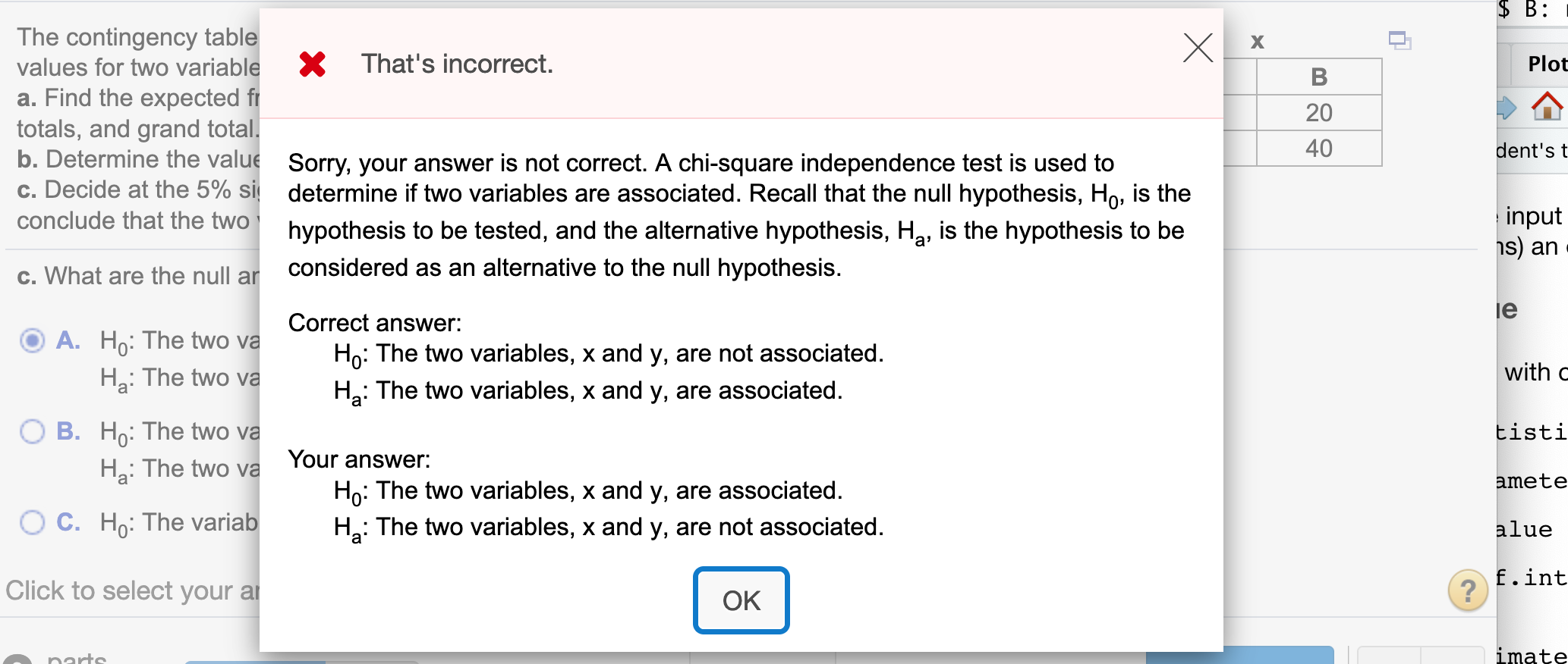
(c). What are the null and alternative hypotheses? Since chi-square statistic test the independence of two variables, the correct hypothesis is
\(H_0:\) The two variables, x and y, are not associated
\(H_a:\) The two variables, x and y, are associated.
Since df = 1, to find critical value for \(\alpha = .51\)
alpha = .05
round(qchisq(1- alpha,1),3)
## [1] 3.841
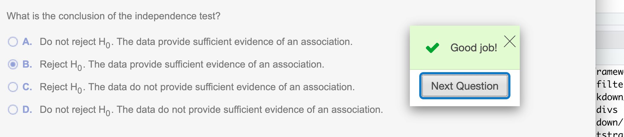
Since \(\chi^2\) is right-tailed test by nature, our test statistic lies in rejected region 30.86 > 3.841 , we have enough evidence to reject the hypothesis
Hope that helps!