13.2.18 chi squaredtest
A distribution and the observed frequencies of the values of a variable from a simple random sample of the population are provided below. Use the chi-square goodness-of-fit test to decide, at the specified significance level, whether the distribution of the variable differs from the given distribution.
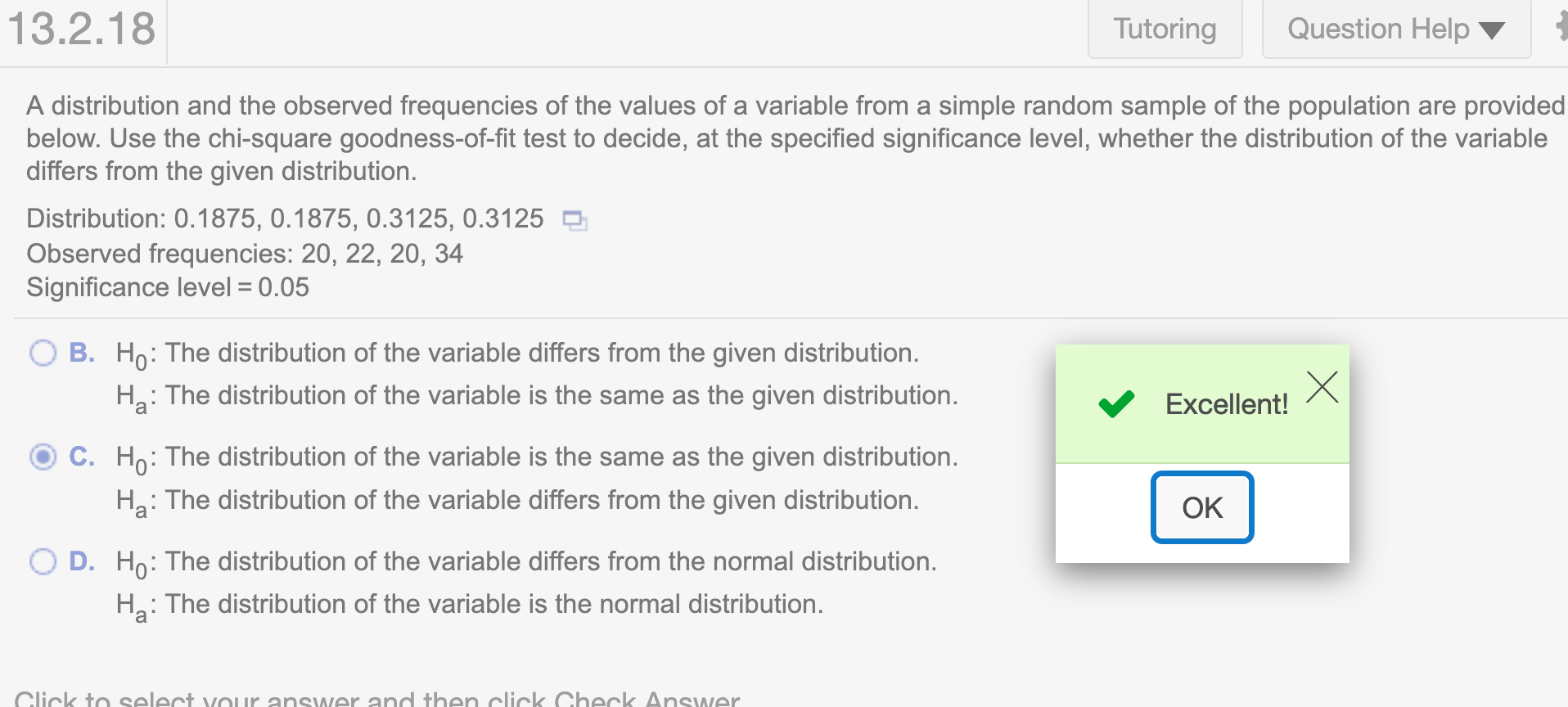
Distribution: 0.1875, 0.1875, 0.3125, 0.3125 Observed frequencies: 20, 22, 20, 34 Significance level = 0.05Determine the null and alternative hypotheses. Choose the correct answer below.
Since the question asks whether the distribution of the variable differs from the given distribution, it is a two-tailed test
\(H_0:\) The distribution of the variable is the same as the given distribution
\(H_a:\) The distribution of the variable differs from given distribution
Compute the value of the test statistic,\(\chi^2\)
First we need to get the data from the question. (We can import it from Excel)
distribution <- c(0.1875, 0.1875, 0.3125, 0.3125)
obFrequency <- c(20, 22, 20, 34)
First approach, we can use chisq.test()
chisq.test(obFrequency,p=distribution, correct=FALSE)##
## Chi-squared test for given probabilities
##
## data: obFrequency
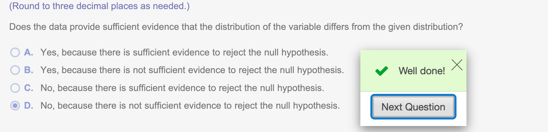
## X-squared = 4.9778, df = 3, p-value = 0.1734Round to 3 decimal places
print(chisq.test(obFrequency,p=distribution, correct=FALSE),6)##
## Chi-squared test for given probabilities
##
## data: obFrequency
## X-squared = 4.978, df = 3, p-value = 0.173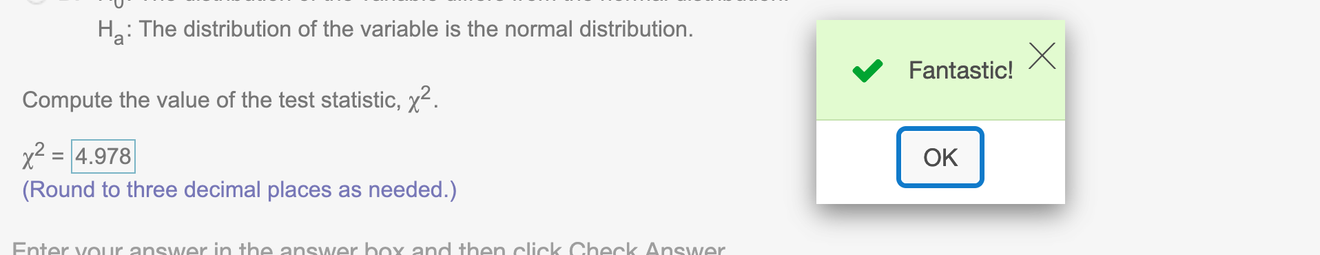
Second approach using formular
We can find the test statistic \(\chi^2\) by using the formula \(\chi^2=\sum{\frac{(O-E)^2}{E}}\)
Expected frequency = sample size * distribution
We can find the sample size by using sum(obFrequency) in R
expFrequency = sum(obFrequency)*distribution
sum((obFrequency-expFrequency)^2/expFrequency)
## [1] 4.977778Round to three decimal places
round(sum((obFrequency-expFrequency)^2/expFrequency),3)## [1] 4.978\(\chi^2\) is right-tailed test by nature
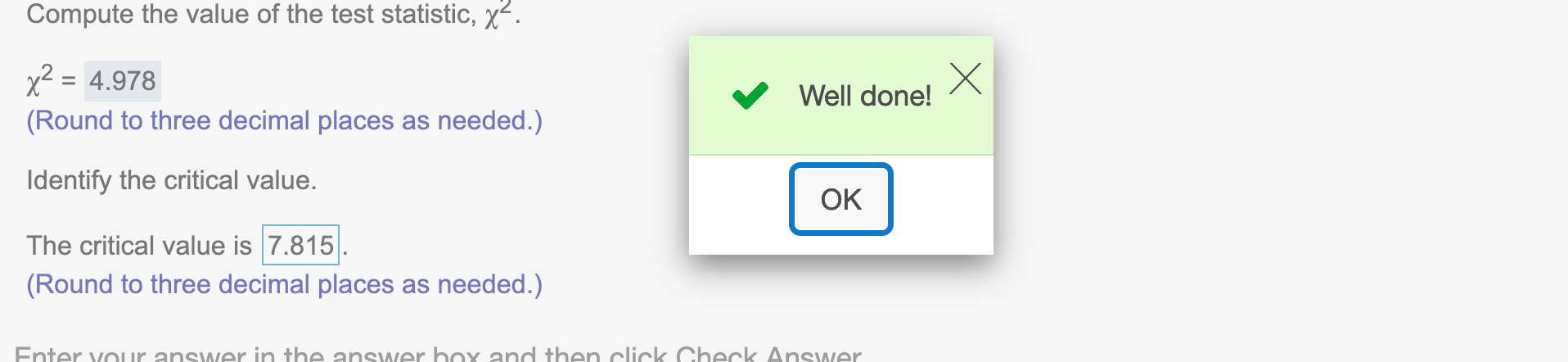
Since we have \(\alpha=.05\) and there are 4 possible values for the variable, so the degree of freedom df = 4 -1 = 3
\(\chi_\alpha^2\) has \(\alpha\) is the area to the right under \(\chi\) curve
We can get \(\chi^2\) value by using the table or we can run qchisq()
qchisq() takes in the area to the left and degree of freedom
alpha = .05
df =  4 - 1
qchisq(1-alpha,df)
## [1] 7.814728Round to three decimal places
round(qchisq(1- alpha,df),3)## [1] 7.815Hope that helps!