16.3.49 one-way ANOVA test
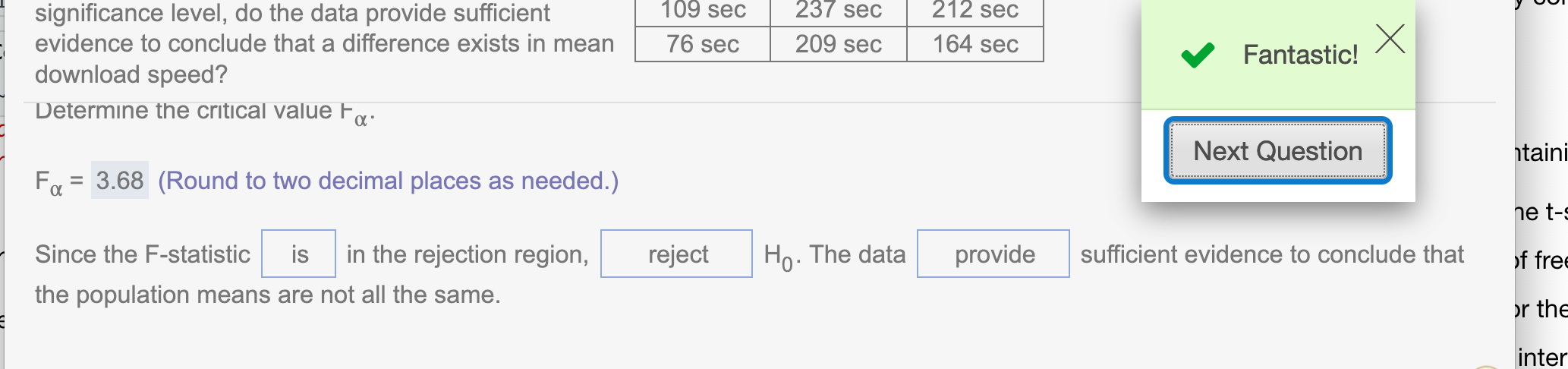
To see how much difference time of day made on the speed at which he could download files, a college sophomore placed a file on a remote server, then proceeded to download it at three different time periods of the day. He downloaded the file 18 times in all, 6 times at each time of day, and recorded the time in seconds that the download took. At the 5% significance level, do the data provide sufficient evidence to conclude that a difference exists in mean download speed?
Notation in one-way ANOVA:
k = number of populations
n = total number of observations
\(\bar x\) = mean of all n observations
\(n_j\) = size of sample from Population j
\(\bar{x_j}\) = mean of sample from Population j
\(s_j^2\) = variance of sample from Population j
\(T_j\) = sum of sample data from Population j
Defining formulas from sums of squares in one-way ANOVA:
SST = \(\sum (x_i - \bar x)^2\)
SSTR = \(\sum n_j(\bar{x_j} - \bar{x})^2\)
SSE = \(\sum (n_j-1)s_j^2\)
One-way ANOVA identity: SST = SSTR + SSE
Computing formulas from sums of squares in one-way ANOVA:
SST = \(\sum x_i^2 - (\sum x_i)^2/n\)
SSTR = \(\sum (T_j^2/n_j) - (\sum x_i)^2/n\)
SSE = SST - SSTR
Mean squares in one-way ANOVA:
MSTR = \(\frac{SSTR}{k-1}\)
MSE = \(\frac{SSE}{n-k}\)
SSE = SST - SSTR
Test statistic for one-way ANOVAA (independent samples, normal populations, and equal population standard deviations):
- F = \(\frac{MSTR}{MSE}\)
with df = (k - 1, n - k)
Confidence interval for \(\mu_i - \mu_j\) in the Tukey multiple-comparison method (independent samples, normal populations, and equal population sstandard deviations):
- \((\bar{x_i} - \bar{x_j}) \pm \frac{q_{\alpha}}{\sqrt{2}}.s\sqrt{\frac{1}{n_i} + \frac{1}{n_j}}\)
where s = \(\sqrt{MSE}\) and \(q_{\alpha}\) is obtained for a q-curve with parameters k and n - k
Test statistic for a Kruskal-Wallis test (independent samples, same-shape populations, all sample sizes 5 or greater):
\(K=\frac{SSTR}{SST/(n-1)}\) or
\(K=\frac{12}{n(n+1)}\sum_{j=1}^{k} \frac{R_j^2}{n_j} - 3(n+1)\)
where SSTR and SST are computed for the ranks of the data, and \(R_j\) denotes the sum of the ranks for the sample data from Population j. K has approximately a chi-square distribution with df = k -1
First, let \(\mu_1, \mu_2,\) and \(\mu_3\) be the population means times for 7 a.m., 5 p.m., and 12 a.m., respectively. What are the correct hypotheses for a one-way ANOVA test?
Since the question asks “At the 5% significance level, do the data provide sufficient evidence to conclude that a difference exists in mean download speed?.” the correct hypothesis is.
\(H_0: \mu_1 = \mu_2 = \mu_3\)
\(H_a:\) Not all the means are equal.
Now conduct a one-way ANOVA test on the data. What is the F-statistic?
First we need to get the data from the question. (We can import it from Excel)
data <- read.csv("https://raw.githubusercontent.com/sileaderwt/MTH1320-UMSL/main/Image%2BData/16.3.49/16.3.49.csv")
data
## Early Evening Late
## 1 70 206 217
## 2 140 293 177
## 3 86 251 176
## 4 209 308 222
## 5 109 237 212
## 6 76 209 164The type of data is tibble in R. To avoid confusion when working with other question, we should create a data frame.
dframe = data.frame(data)
dframe
## Early Evening Late
## 1 70 206 217
## 2 140 293 177
## 3 86 251 176
## 4 209 308 222
## 5 109 237 212
## 6 76 209 164First approach: using anova() in R which Professor Covert introduces in the video lectures (recommended)
X <- c()
len <- c()
for(item in dframe){
  X <- c(X, item[!is.na(item)])
  len <- c(len, length(item[!is.na(item)]))
}
X
## [1] 70 140 86 209 109 76 206 293 251 308 237 209 217 177 176 222 212 164len## [1] 6 6 6We import name of our data.
Y= rep(names(dframe), times = len)
Y
## [1] "Early" "Early" "Early" "Early" "Early" "Early" "Evening"
## [8] "Evening" "Evening" "Evening" "Evening" "Evening" "Late" "Late"
## [15] "Late" "Late" "Late" "Late"dframe2 = data.frame(X,Y)
dframe2## X Y
## 1 70 Early
## 2 140 Early
## 3 86 Early
## 4 209 Early
## 5 109 Early
## 6 76 Early
## 7 206 Evening
## 8 293 Evening
## 9 251 Evening
## 10 308 Evening
## 11 237 Evening
## 12 209 Evening
## 13 217 Late
## 14 177 Late
## 15 176 Late
## 16 222 Late
## 17 212 Late
## 18 164 LateWe run anova()
fm1 = aov(X~Y, data=dframe2)
fm1
## Call:
## aov(formula = X ~ Y, data = dframe2)
##
## Terms:
## Y Residuals
## Sum of Squares 55776.44 26028.67
## Deg. of Freedom 2 15
##
## Residual standard error: 41.65627
## Estimated effects may be unbalancedanova(fm1)## Analysis of Variance Table
##
## Response: X
## Df Sum Sq Mean Sq F value Pr(>F)
## Y 2 55776 27888.2 16.072 0.0001862 ***
## Residuals 15 26029 1735.2
## ---
## Signif. codes: 0 '***' 0.001 '**' 0.01 '*' 0.05 '.' 0.1 ' ' 1We can run str() to see structure of our data. We can extract any data from the frame.
str(anova(fm1))## Classes 'anova' and 'data.frame': 2 obs. of 5 variables:
## $ Df : int 2 15
## $ Sum Sq : num 55776 26029
## $ Mean Sq: num 27888 1735
## $ F value: num 16.1 NA
## $ Pr(>F) : num 0.000186 NA
## - attr(*, "heading")= chr [1:2] "Analysis of Variance Table\n" "Response: X"Round to 2 decimal places
print((anova(fm1)$`F value`), 4)## [1] 16.07 NA
Now determine the critical value \(F_{\alpha}\)
Since \(\alpha = .05\), df(2,15)
qf(1-.05, 2, 15)## [1] 3.68232Round to decimal places
round(qf(1-.05, 2, 15), 2)## [1] 3.68
Since our test statistic = 16.07 > our critical value \(F_{\alpha}=3.68\) and it is a right-tailed test, we have enough evidence to reject the hypothesis.
Second approach: using the formula from the book
The same approach with question 16.3.43, we could see that two approaches have the same answer
(a) Compute SST, SSTR, and SSE using the following computing formulas, where xi is the ith observation, n is the total number of observations, nj is the sample size for population j, and Tj is the sum of the sample data from population j.
Names of variables
\(\sum{x}: Sx\)
\(\sum x^2: Sxx\) \(\sum (T_j^2/n_j)\): T
n = total number of observations: n
To make it easy to find \(\sum x\), we store all data into a variable x
x <- c()
for(item in dframe){
  x <- c(x, item[!is.na(item)])
}
x
## [1] 70 140 86 209 109 76 206 293 251 308 237 209 217 177 176 222 212 164n = length(x)
n## [1] 18Find \(\sum x_i\)
sum(x)## [1] 3362Find \(\sum x_i^2\)
sum(x*x)## [1] 709752Find SST
To find SST, we use formula SST = \(\sum x_i^2 - (\sum x_i)^2/n\)
SST = sum(x*x) - (sum(x))^2/n
SST
## [1] 81805.11Find \(\sum (T_j^2/n_j)\)
T = 0
for(item in dframe){
  t =  item[!is.na(item)]
  T = T + sum(t)^2/length(t)
}
T
## [1] 683723.3Find SSTR, we use formula SSTR = \(\sum (T_j^2/n_j) - (\sum x_i)^2/n\)
SSTR = T - sum(x)^2/n
SSTR
## [1] 55776.44Find SSE, we use formula SSE = SST - SSTR
SSE = SST - SSTR
SSE
## [1] 26028.67(b). Compare your results in part (a) for SSTR and SSE with the following results from the defining formulas.
We find SSTR, SSE, SST by using defining formula
Find SST using the formula SST = \(\sum (x_i - \bar x)^2\)
SST = sum(x*x) - (sum(x))^2/n
SST
## [1] 81805.11Find SSTR using the formula SSTR = \(\sum n_j(\bar{x_j} - \bar{x})^2\)
SSTR = 0
for(item in dframe){
  t =  item[!is.na(item)]
  SSTR = SSTR + length(t)*(mean(t) - mean(x))^2
}
SSTR
## [1] 55776.44Find SSE using the formula SSE = \(\sum (n_j-1)s_j^2\)
SSE = 0
for(item in dframe){
  t =  item[!is.na(item)]
  SSE = SSE + (length(t)-1)*sd(t)^2
}
SSE
## [1] 26028.67(c) Construct a one-way ANOVA table.
Find df treatment
k = length(dframe)
k-1
## [1] 2Find SS treatment
SSTR## [1] 55776.44Find MS treatment
MSTR = SSTR/(k-1)
MSTR
## [1] 27888.22Find Error df
n - k## [1] 15Find Error SS
SSE## [1] 26028.67Find Error MS
MSE = SSE / (n - k)
MSE
## [1] 1735.244Find F-statistic treatment
MSTR / MSE## [1] 16.07164Find df total
n - 1## [1] 17Find SS total
SST## [1] 81805.11Now determine the critical value \(F_{\alpha}\)
Since \(\alpha = .05\)
alpha = 0.05
qf(1-alpha, k-1, n-k)
## [1] 3.68232Round to decimal places
round(qf(1-alpha, k-1, n-k), 2)## [1] 3.68Hope that helps!