10.5.157 paired t-test left-tailed
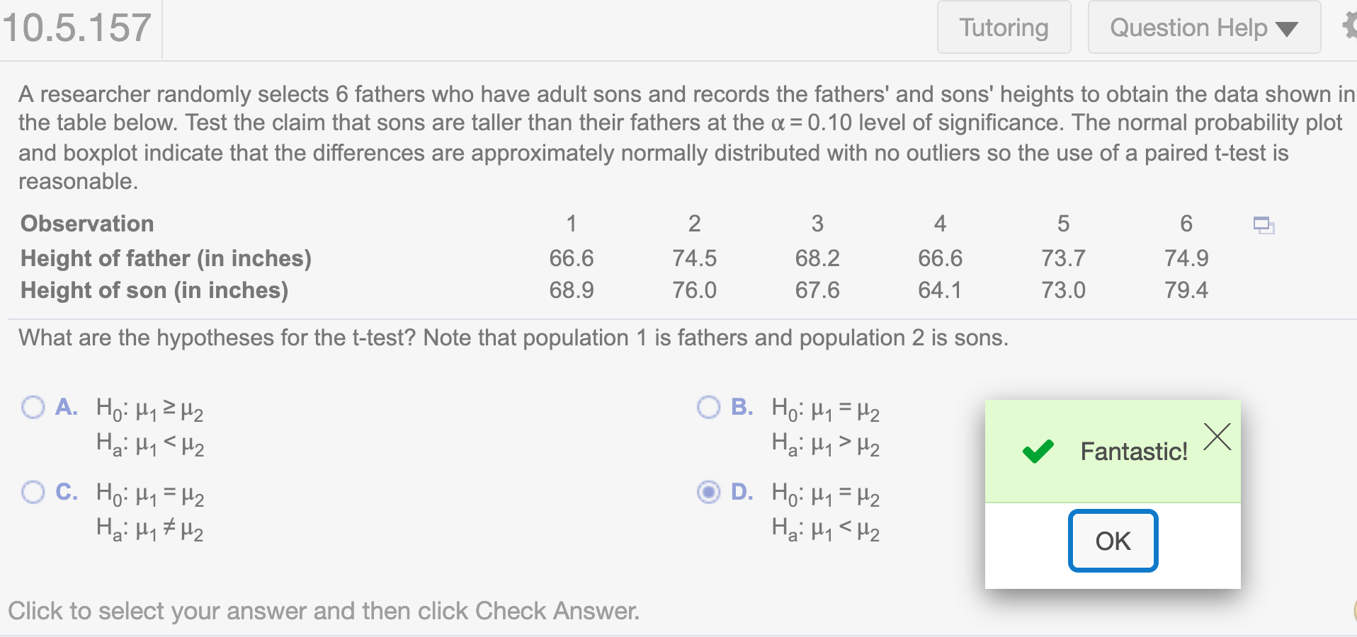
A researcher randomly selects 6 fathers who have adult sons and records the fathers’ and sons’ heights to obtain the data shown in the table below. Test the claim that sons are taller than their fathers at the \(\alpha =\) 0.10 level of significance. The normal probability plot and boxplot indicate that the differences are approximately normally distributed with no outliers so the use of a paired t-test is reasonable.
What are the hypotheses for the t-test? Note that population 1 is fathers and population 2 is sons.
Since test the claim that sons are taller than their fathers, we have left-tailed test
\(H_0:\mu_1 = \mu_2\)
\(H_a:\mu_1 < \mu_2\)
First, we need to get the data from the question. (We could import the data from Excel)
father <- c(66.6, 74.5, 68.2, 66.6, 73.7, 74.9)
son <- c(68.9, 76.0, 67.6, 64.1, 73.0, 79.4)
Use population 1 minus population 2 as the difference.
We store difference between father and son in variable difference and run test statistic. Since \(\alpha = .10\) we have confidence level = .9 First approach use t.test()
difference = father - son
t.test(difference, conf.level = .9, alternative = "less")
##
## One Sample t-test
##
## data: difference
## t = -0.73175, df = 5, p-value = 0.2486
## alternative hypothesis: true mean is less than 0
## 90 percent confidence interval:
## -Inf 0.7626912
## sample estimates:
## mean of x
## -0.75Round to 3 decimal places
print(t.test(difference, conf.level = .9, alternative = "less"),5)##
## One Sample t-test
##
## data: difference
## t = -0.732, df = 5, p-value = 0.25
## alternative hypothesis: true mean is less than 0
## 90 percent confidence interval:
## -Inf 0.76269
## sample estimates:
## mean of x
## -0.75Since we have 6 pairs of data, our degree of freedom is 6 - 1 = 5 and we have left-tailed test with \(\alpha = .1\), the area to the left of critical value = \(\alpha\)
round(qt(.1, 5), 3)## [1] -1.476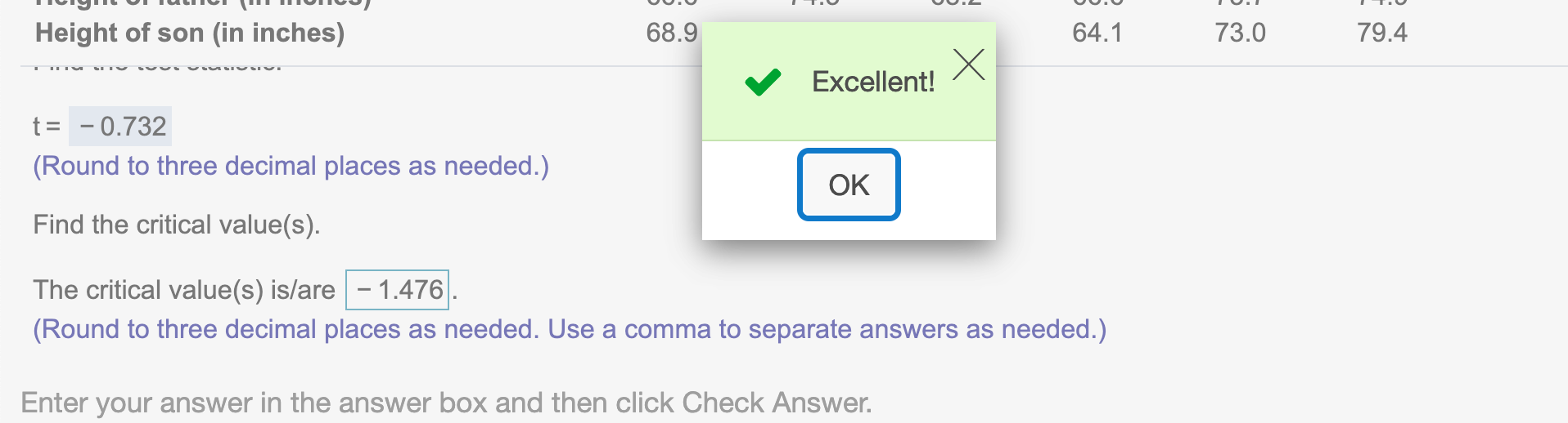
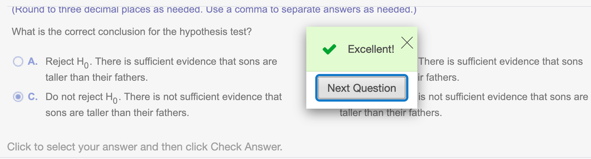
Since the test statistic value t = -0.732 is larger than the critical value \(t_{\alpha} = -1.476\), we do not have enough evidence to reject hypothesis.
Second appraach to find test statistic, we can use formula \(t=\frac{\bar d}{\frac{s_d}{\sqrt{n}}}\)
n = 6
mean(difference)/(sd(difference)/sqrt(n))
## [1] -0.7317508Round to 3 decimal places
round(mean(difference)/(sd(difference)/sqrt(n)),3)## [1] -0.732Hope that helps!