16.3.43 ANOVA table
The data shown to the right are from independent simple random samples from three populations. Use these data to complete parts (a) through (d).
Notation in one-way ANOVA:
k = number of populations
n = total number of observations
\(\bar x\) = mean of all n observations
\(n_j\) = size of sample from Population j
\(\bar{x_j}\) = mean of sample from Population j
\(s_j^2\) = variance of sample from Population j
\(T_j\) = sum of sample data from Population j
Defining formulas from sums of squares in one-way ANOVA:
SST = \(\sum (x_i - \bar x)^2\)
SSTR = \(\sum n_j(\bar{x_j} - \bar{x})^2\)
SSE = \(\sum (n_j-1)s_j^2\)
One-way ANOVA identity: SST = SSTR + SSE
Computing formulas from sums of squares in one-way ANOVA:
SST = \(\sum x_i^2 - (\sum x_i)^2/n\)
SSTR = \(\sum (T_j^2/n_j) - (\sum x_i)^2/n\)
SSE = SST - SSTR
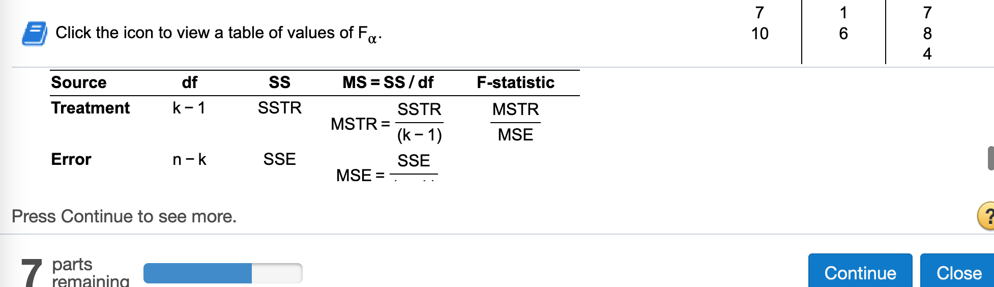
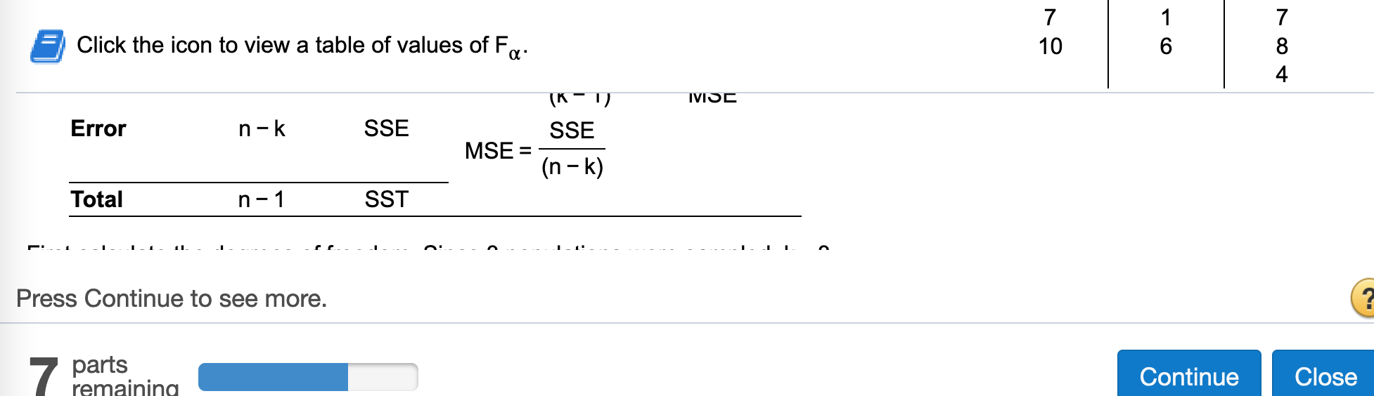
Mean squares in one-way ANOVA:
MSTR = \(\frac{SSTR}{k-1}\)
MSE = \(\frac{SSE}{n-k}\)
SSE = SST - SSTR
Test statistic for one-way ANOVAA (independent samples, normal populations, and equal population standard deviations):
- F = \(\frac{MSTR}{MSE}\)
with df = (k - 1, n - k)
Confidence interval for \(\mu_i - \mu_j\) in the Tukey multiple-comparison method (independent samples, normal populations, and equal population sstandard deviations):
- \((\bar{x_i} - \bar{x_j}) \pm \frac{q_{\alpha}}{\sqrt{2}}.s\sqrt{\frac{1}{n_i} + \frac{1}{n_j}}\)
where s = \(\sqrt{MSE}\) and \(q_{\alpha}\) is obtained for a q-curve with parameters k and n - k
Test statistic for a Kruskal-Wallis test (independent samples, same-shape populations, all sample sizes 5 or greater):
\(K=\frac{SSTR}{SST/(n-1)}\) or
\(K=\frac{12}{n(n+1)}\sum_{j=1}^{k} \frac{R_j^2}{n_j} - 3(n+1)\)
where SSTR and SST are computed for the ranks of the data, and \(R_j\) denotes the sum of the ranks for the sample data from Population j. K has approximately a chi-square distribution with df = k -1
First approach: Using formulas from the book
(a) Compute SST, SSTR, and SSE using the following computing formulas, where \(x_i\) is the ith observation, n is the total number of observations, \(n_j\) is the sample size for population j, and \(T_j\) is the sum of the sample data from population j.
First we need to get the data from the question. (We can import it from Excel)
data <- read.csv("https://raw.githubusercontent.com/sileaderwt/MTH1320-UMSL/main/Image%2BData/16.3.43/16.3.43.csv")
data
## Sample1 Sample2 Sample3
## 1 6 2 1
## 2 5 3 4
## 3 4 1 2
## 4 NA NA 5The type of data is tibble in R. To avoid confusion when working with other question, we should create a data frame.
dframe = data.frame(data)
dframe
## Sample1 Sample2 Sample3
## 1 6 2 1
## 2 5 3 4
## 3 4 1 2
## 4 NA NA 5Names of variables
\(\sum{x}: Sx\)
\(\sum x^2: Sxx\) \(\sum (T_j^2/n_j)\): T
n = total number of observations: n
To make it easy to find \(\sum x\), we store all data into a variable x
x <- c()
for(item in dframe){
  x <- c(x, item[!is.na(item)])
}
x
## [1] 6 5 4 2 3 1 1 4 2 5n = length(x)
n## [1] 10Find \(\sum x_i\)
sum(x)## [1] 33Find \(\sum x_i^2\)
sum(x*x)## [1] 137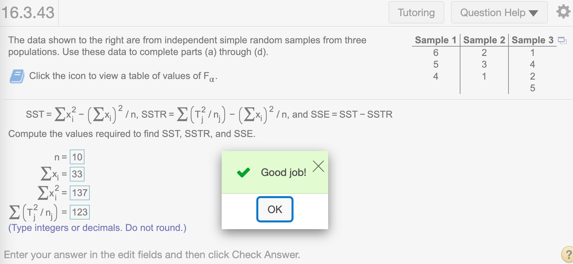
Find SST
To find SST, we use formula SST = \(\sum x_i^2 - (\sum x_i)^2/n\)
SST = sum(x*x) - (sum(x))^2/n
SST
## [1] 28.1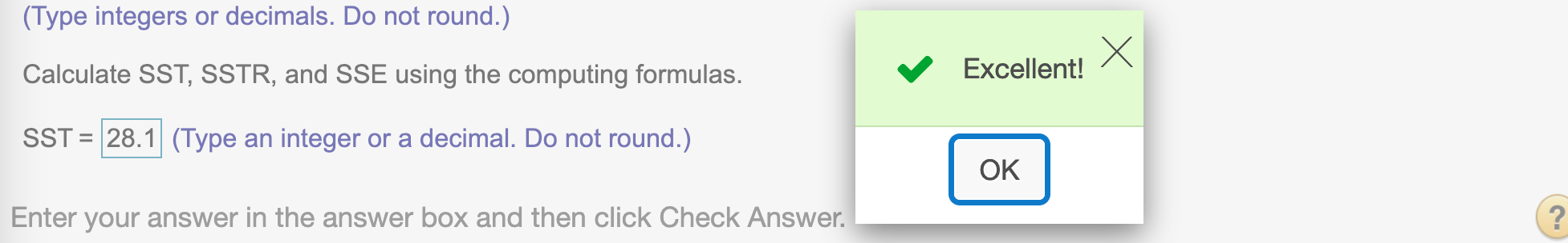
Find \(\sum (T_j^2/n_j)\)
T = 0
for(item in dframe){
  t =  item[!is.na(item)]
  T = T + sum(t)^2/length(t)
}
T
## [1] 123Find SSTR, we use formula SSTR = \(\sum (T_j^2/n_j) - (\sum x_i)^2/n\)
SSTR = T - sum(x)^2/n
SSTR
## [1] 14.1
Find SSE, we use formula SSE = SST - SSTR
SSE = SST - SSTR
SSE
## [1] 14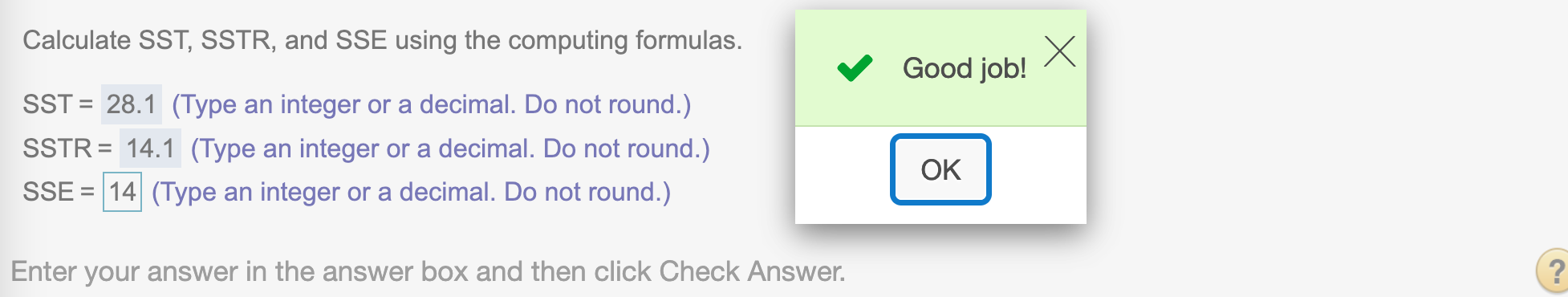
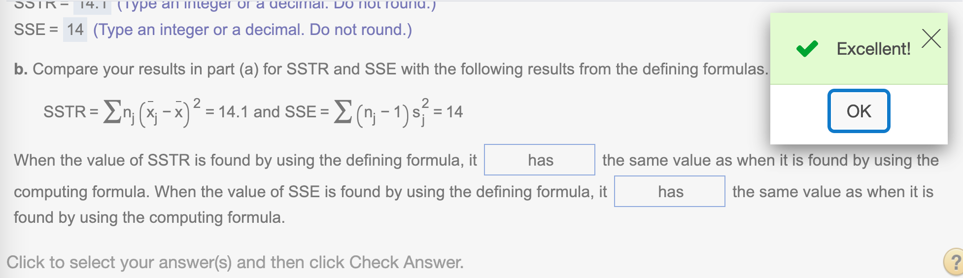
(b). Compare your results in part (a) for SSTR and SSE with the following results from the defining formulas.
We find SSTR, SSE, SST by using defining formula
Find SST using the formula SST = \(\sum (x_i - \bar x)^2\)
SST = sum(x*x) - (sum(x))^2/n
SST
## [1] 28.1Find SSTR using the formula SSTR = \(\sum n_j(\bar{x_j} - \bar{x})^2\)
SSTR = 0
for(item in dframe){
  t =  item[!is.na(item)]
  SSTR = SSTR + length(t)*(mean(t) - mean(x))^2
}
SSTR
## [1] 14.1Find SSE using the formula SSE = \(\sum (n_j-1)s_j^2\)
SSE = 0
for(item in dframe){
  t =  item[!is.na(item)]
  SSE = SSE + (length(t)-1)*sd(t)^2
}
SSE
## [1] 14We have the same answer by using two different formulas.
(c) Construct a one-way ANOVA table.
Find df treatment
k = length(dframe)
k-1
## [1] 2Find SS treatment
SSTR## [1] 14.1Find MS treatment
MSTR = SSTR/(k-1)
MSTR
## [1] 7.05Find Error df
n - k## [1] 7Find Error SS
SSE## [1] 14Find Error MS
MSE = SSE / (n - k)
MSE
## [1] 2Find F-statistic treatment
MSTR / MSE## [1] 3.525Find df total
n - 1## [1] 9Find SS total
SST## [1] 28.1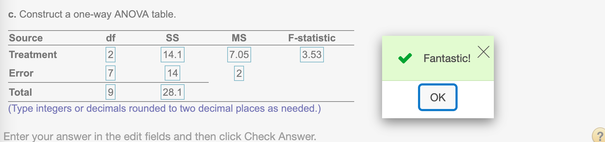
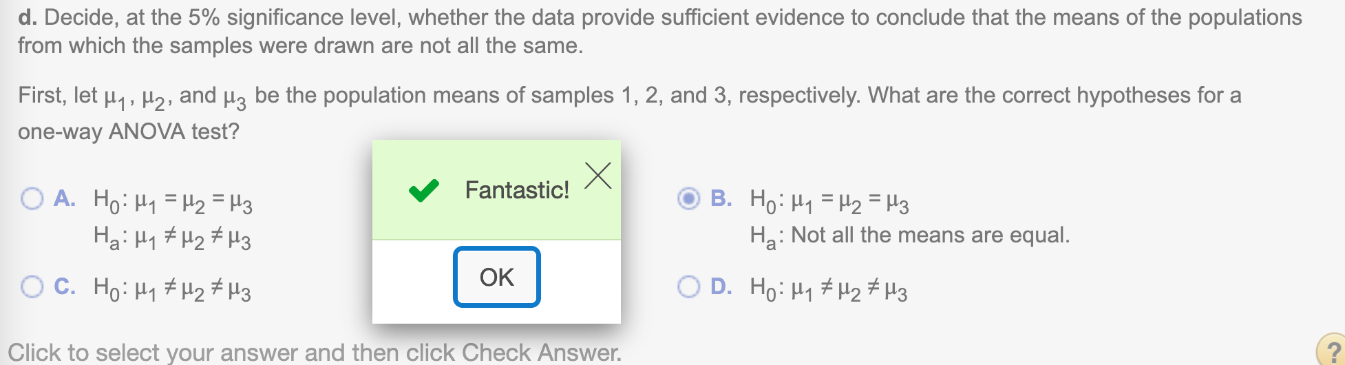
(d) Decide, at the 5% significance level, whether the data provide sufficient evidence to conclude that the means of the populations from which the samples were drawn are not all the same.
First, let \(\mu_1, \mu_2,\) and \(\mu_3\)be the population means of samples 1, 2, and 3, respectively. What are the correct hypotheses for a one-way ANOVA test?
\(H_0: \mu_1 = \mu_2 = \mu_3\)
\(H_a:\) Not all the means are equal.
Now determine the critical value \(F_{\alpha}\)
Since \(\alpha = .05\)
alpha = 0.05
qf(1-alpha, k-1, n-k)
## [1] 4.737414Round to decimal places
round(qf(1-alpha, k-1, n-k), 2)## [1] 4.74
Since our test statistic = 3.53 < our critical value \(F_{\alpha}=4.74\) and it is a right-tailed test, we do not have enough evidence to reject the hypothesis.
Second approach: using anova() in R which Professor Covert introduces in the video lectures (recommended)
X <- c()
len <- c()
for(item in dframe){
  X <- c(X, item[!is.na(item)])
  len <- c(len, length(item[!is.na(item)]))
}
X
## [1] 6 5 4 2 3 1 1 4 2 5len## [1] 3 3 4We import name of our data.
Y= rep(names(dframe), times = len)
Y
## [1] "Sample1" "Sample1" "Sample1" "Sample2" "Sample2" "Sample2" "Sample3"
## [8] "Sample3" "Sample3" "Sample3"dframe2 = data.frame(X,Y)
dframe2## X Y
## 1 6 Sample1
## 2 5 Sample1
## 3 4 Sample1
## 4 2 Sample2
## 5 3 Sample2
## 6 1 Sample2
## 7 1 Sample3
## 8 4 Sample3
## 9 2 Sample3
## 10 5 Sample3We run anova()
fm1 = aov(X~Y, data=dframe2)
fm1
## Call:
## aov(formula = X ~ Y, data = dframe2)
##
## Terms:
## Y Residuals
## Sum of Squares 14.1 14.0
## Deg. of Freedom 2 7
##
## Residual standard error: 1.414214
## Estimated effects may be unbalancedanova(fm1)## Analysis of Variance Table
##
## Response: X
## Df Sum Sq Mean Sq F value Pr(>F)
## Y 2 14.1 7.05 3.525 0.08729 .
## Residuals 7 14.0 2.00
## ---
## Signif. codes: 0 '***' 0.001 '**' 0.01 '*' 0.05 '.' 0.1 ' ' 1We can run str() to see structure of our data. We can extract any data from the frame.
str(anova(fm1))## Classes 'anova' and 'data.frame': 2 obs. of 5 variables:
## $ Df : int 2 7
## $ Sum Sq : num 14.1 14
## $ Mean Sq: num 7.05 2
## $ F value: num 3.52 NA
## $ Pr(>F) : num 0.0873 NA
## - attr(*, "heading")= chr [1:2] "Analysis of Variance Table\n" "Response: X"Print F-statistic value to 2 decimal places
print((anova(fm1)$`F value`), 3)## [1] 3.52 NAFind df of treatment and error
anova(fm1)$`Df`## [1] 2 7Find SS of treatment and error to 2 decimal places
print((anova(fm1)$`Sum Sq`), 4)## [1] 14.1 14.0Find MS of treatment and error to 2 decimal places
print((anova(fm1)$`Mean Sq`), 3)## [1] 7.05 2.00Find P-value to 2 decimal places
print((anova(fm1)$`Pr(>F)`), 3)## [1] 0.0873 NATwo approaches give the same answer. The second approach is recommended since professor Covert introduces in the video lecture.
Now determine the critical value \(F_{\alpha}\)
Since \(\alpha = .05\), df(2,7)
qf(1-.05, 2, 7)## [1] 4.737414Round to decimal places
round(qf(1-.05, 2, 7), 2)## [1] 4.74Hope that helps!